CSV Dataset Summarizer

In this tutorial we will build a CSV dataset summarizer — a web app where you upload any CSV file and immediately get a structured overview of what’s inside.

No code, no terminal, no pandas knowledge required from the user. Just upload and read.

We will use:

• pandas for reading and analysing the CSV
• skrub for the interactive data preview table
• Mercury to turn the notebook into a web app

The full notebook code is available in our GitHub repository.

You can also try the live demo.

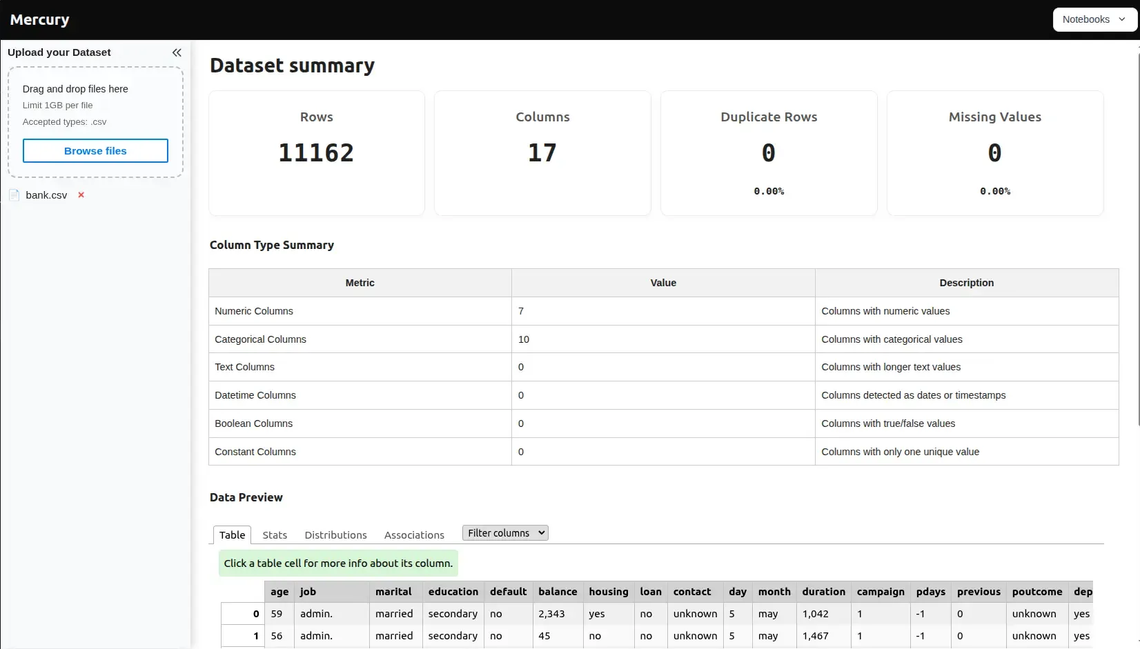
What the app shows

After the user uploads a CSV, the app displays three sections:

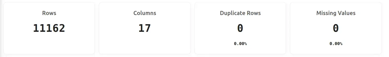
1. Key indicators — rows, columns, duplicate rows (with %), missing values (with %)
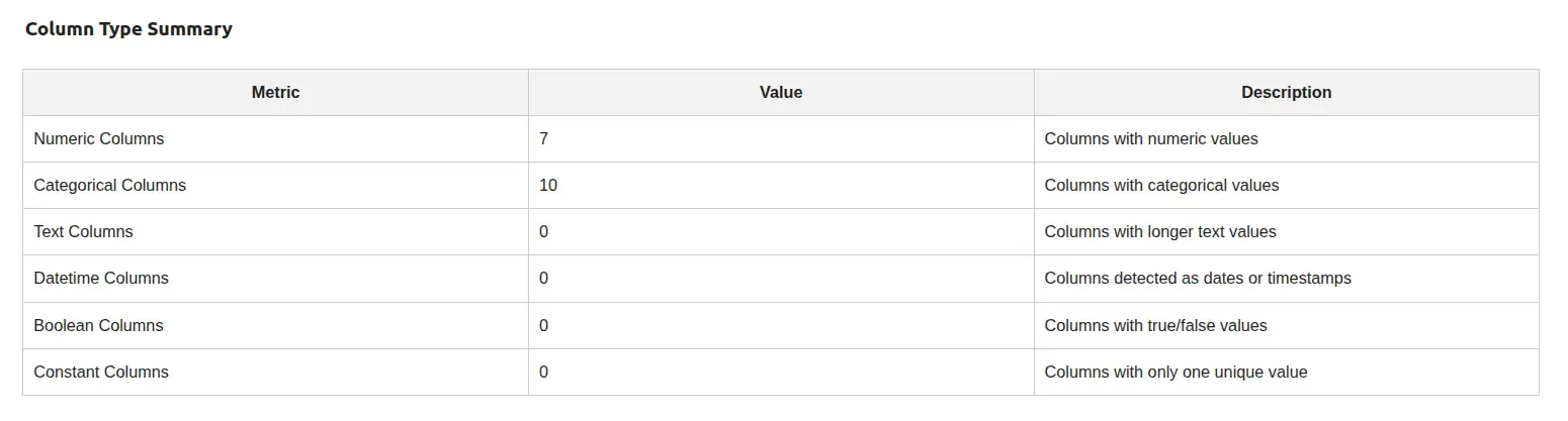
2. Column type summary — a table breaking down how many columns are numeric, categorical, text, datetime, boolean, or constant
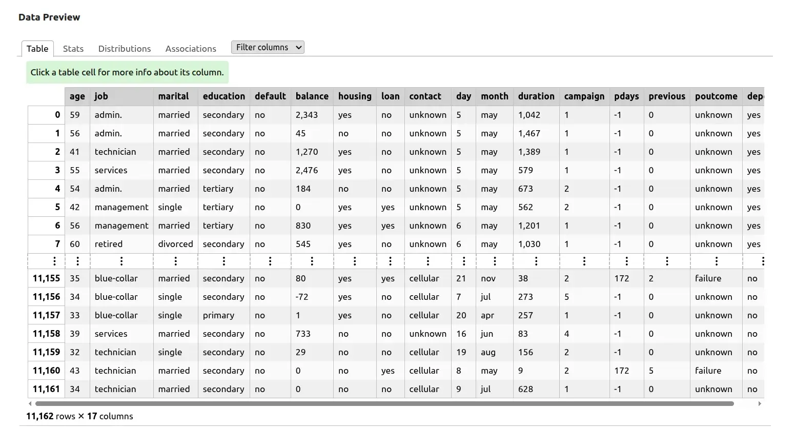
3. Data preview — an interactive table with the first 15 rows, powered by skrub’s TableReport

1. Install packages

pip install mercury pandas skrub

2. Import libraries

import mercury as mr
from IPython.display import clear_output

Note

clear_output from IPython is used to hide empty cells when no file has been uploaded yet, keeping the app clean on first load.

3. Add a welcome message

welcome_md = mr.Markdown("# Upload the dataset and check the summary")

This message is shown before the user uploads anything. Once a file is uploaded, it gets replaced by the actual summary title.

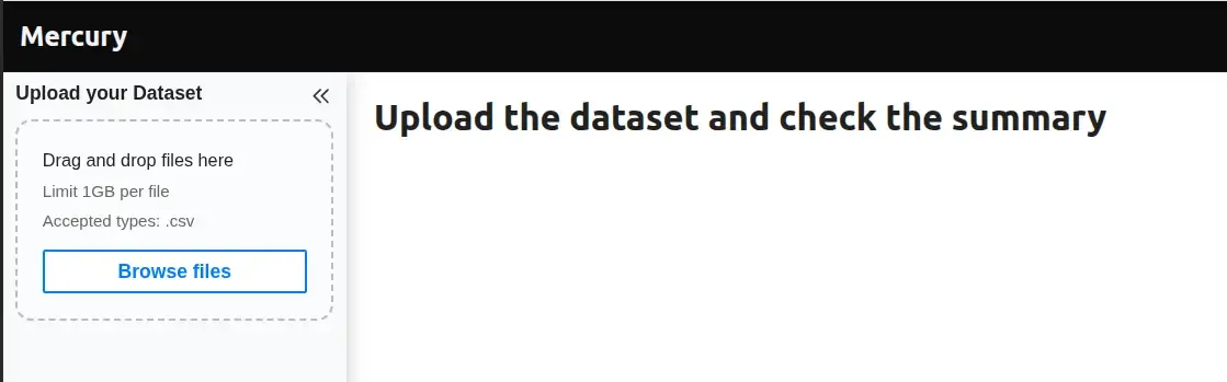
4. Add the file upload widget

input_file = mr.UploadFile(label="Upload your Dataset", accept='.csv', max_file_size='1GB')

UploadFile renders a file picker in the app sidebar. We restrict it to .csv files and allow up to 1 GB.

When the user picks a file:

• input_file.name becomes the filename (non-empty string)
• input_file.value contains the raw file bytes

Mercury automatically re-runs the notebook when the upload changes, so all cells below react immediately.

5. Read the CSV

if input_file.name is not None:
    import pandas as pd
    from io import BytesIO
    from skrub import TableReport
    data = BytesIO(input_file.value)
    df = pd.read_csv(data)

We wrap the raw bytes in BytesIO so pandas can read them directly, without saving the file to disk first.

6. Compute the summary statistics

if input_file.name is not None:
    # shape
    row_count = df.shape[0]
    col_count = df.shape[1]

    # missing values
    missing_count = df.isna().sum().sum()
    missing_procent = df.isna().mean().mean() * 100

    # duplicates
    duplicates_count = df.duplicated().sum()
    duplicates_procent = (duplicates_count / row_count) * 100

Straightforward pandas — nothing unusual here. We keep both the raw counts and percentages so we can show both in the indicators.

7. Detect column types

This is the most interesting part of the app. We go beyond pandas’ built-in dtypes to catch edge cases.

    # basic pandas types
    numeric_columns   = df.select_dtypes(include=["number"]).columns.tolist()
    boolean_columns   = df.select_dtypes(include=["bool"]).columns.tolist()
    datetime_columns  = df.select_dtypes(include=["datetime", "datetimetz"]).columns.tolist()
    object_columns    = df.select_dtypes(include=["object", "category"]).columns.tolist()

Detecting dates stored as text

A very common real-world problem: date columns that look like "2024-01-15" but are stored as plain strings. Pandas reads them as object dtype and misses them. We catch them manually:

    detected_datetime_columns = []
    for col in object_columns:
        converted = pd.to_datetime(df[col], errors="coerce")
        valid_ratio = converted.notna().mean()
        if valid_ratio > 0.8:
            detected_datetime_columns.append(col)

    datetime_columns = list(set(datetime_columns + detected_datetime_columns))

If more than 80% of values in a column parse as a valid date, we treat it as datetime.

Detecting free-text columns

Long string columns (descriptions, comments, addresses) shouldn’t be counted as categorical. We separate them out by average string length:

    text_columns = []
    for col in object_columns:
        if col not in datetime_columns:
            avg_text_length = df[col].dropna().astype(str).str.len().mean()
            if avg_text_length > 30:
                text_columns.append(col)

Constant columns

Columns with only one unique value carry no information and are worth flagging:

    constant_columns = [
        col for col in all_columns
        if df[col].nunique(dropna=False) <= 1
    ]

Categorical columns

Everything that doesn’t fall into numeric, boolean, datetime, or text:

    excluded_from_categorical = set(
        datetime_columns + text_columns + boolean_columns + numeric_columns
    )
    categorical_columns = [
        col for col in all_columns
        if col not in excluded_from_categorical
    ]

8. Build the output widgets

Indicators

    ind_basic = mr.Indicator([
        mr.Indicator(value=row_count,         label="Rows"),
        mr.Indicator(value=col_count,         label="Columns"),
        mr.Indicator(value=duplicates_count,  label="Duplicate Rows",  delta=f"{duplicates_procent:.2f}%"),
        mr.Indicator(value=missing_count,     label="Missing Values",  delta=f"{missing_procent:.2f}%"),
    ])

Indicator displays a big number with an optional delta label below it. Nesting multiple Indicator objects inside one renders them side by side.

Column type table

    dane = {
        "Metric": ["Numeric Columns", "Categorical Columns", "Text Columns",
                   "Datetime Columns", "Boolean Columns", "Constant Columns"],
        "Value":  [len(numeric_columns), len(categorical_columns), len(text_columns),
                   len(datetime_columns), len(boolean_columns), len(constant_columns)],
        "Description": [
            "Columns with numeric values",
            "Columns with categorical values",
            "Columns with longer text values",
            "Columns detected as dates or timestamps",
            "Columns with true/false values",
            "Columns with only one unique value",
        ]
    }
    tabelka = mr.Table(dane)

Table renders a plain dict or DataFrame as a clean HTML table.

Data preview

    report = TableReport(df, n_rows=15)
    display(report)

TableReport from skrub renders an interactive table with per-column statistics, sortable headers, and value distributions. It does a lot of work for one line of code.

9. Conditional display

The last cells use a simple pattern to show the right content depending on whether a file has been uploaded:

if input_file.name is None:
    display(welcome_md)
else:
    display(title_md)

if input_file.name is not None:
    display(ind_basic)
else:
    clear_output(wait=False)

The same pattern repeats for the column type table and data preview. clear_output() hides the cell output entirely when there’s nothing to show, so the app doesn’t leave empty gaps on first load.

10. Run as a web app

Start the Mercury server from the folder containing the notebook:

mercury

Mercury will detect all *.ipynb files and serve them as web applications.

Notes and tips

• The 80% threshold for datetime detection works well in practice, but you can tune it for stricter or looser detection.
• The text column threshold of 30 characters is a heuristic. Short categoricals like country names average well under 30; free-text fields like comments average well above.
• TableReport can be slow on very large files. Consider adding df = df.sample(10_000) before calling it if you expect datasets with hundreds of thousands of rows.
• To support Excel files as well, add accept='.csv,.xlsx' to UploadFile and handle both formats with pd.read_csv / pd.read_excel based on input_file.name.